Adding Confidence to Large‑Language‑Model Classifiers
Large language models are astonishingly good at zero‑shot and few‑shot classification, but how sure is the model? Learn how to turn hidden signals into well‑calibrated confidence scores your business can trust.
Adding Confidence to Large‑Language‑Model Classifiers
Large language models (LLMs) are astonishingly good at zero‑shot and few‑shot classification: from flagging toxic comments to routing support tickets. Yet the first question our clients ask after the demo is, "How sure is the model?"
In regulated, customer‑facing, or high‑risk domains, a raw label isn't enough-you need a probability you can put in a risk matrix, a QA workflow, or a dashboard. Below we show how to turn the signals hidden inside every LLM into well‑calibrated confidence scores your business can trust.
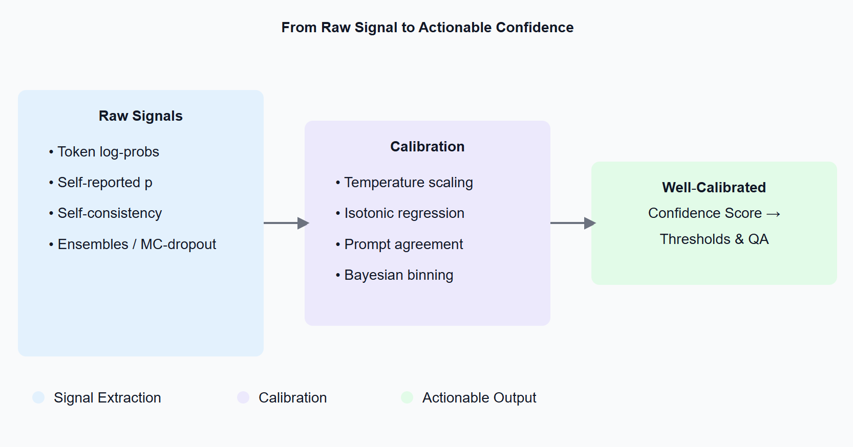
Confidence Measures Diagram
1 The stakes: why confidence matters
Imagine a customs‑clearance workflow that auto‑classifies goods descriptions. A 90 %‑certain misclassification triggers a manual review; a 99 %‑certain one sails through. Without calibrated probabilities you either flood humans with false alarms or, worse, let costly errors slip through. Confidence scores turn 'black‑box magic' into an auditable component of your decision pipeline.
2 Where do confidence signals come from?
Token log‑probabilities. Most model APIs (OpenAI, Anthropic, Mistral, llama‑cpp, …) return logprobs if you set the flag. Aggregate the probability mass assigned to each class token-that's your raw score.
Self‑reported probabilities. You can simply ask: "Give the label and a probability between 0 and 1." The model will oblige-surprisingly well, but usually over‑confident.
Self‑consistency sampling. Re‑prompt or sample the model several times. If the answers disagree, treat it as uncertainty (see SelfCheckGPT).
Ensembles & MC‑dropout. Classical model‑uncertainty tricks still work: run multiple checkpoints or enable dropout at inference to get a distribution of logits.
3 From raw scores to reliable numbers: calibration 101
LLMs tend to be mis‑calibrated out of the box (the 80 %‑confidence bucket might only be right 60 % of the time). Post‑hoc calibration fixes that:
- Temperature/Platt scaling – learn one scalar T on a validation set; divide logits by T.
- Isotonic regression – a non‑parametric monotone mapping for multi‑class tasks.
- Prompt‑agreement calibration – average log‑probs across diverse templates.
- Bayesian binning or ensemble temperature scaling – best for safety‑critical domains.
Evaluate with Expected Calibration Error (ECE) or Brier score; aim for ECE < 2 % on held‑out data.
4 Hands‑on: Calibrating a zero‑shot spam classifier
The snippet below shows the essence:
import openai, numpy as np, json, math

LABELS = { "A": "spam", "B": "not spam" }

def classify(text, T=1.0):
   prompt = f"Classify the following text as A) spam or B) not spam.\nTEXT: {text}\nAnswer with a single letter."
   resp = openai.ChatCompletion.create(
       model="gpt-4o-mini",
       messages=[{ "role": "user", "content": prompt }],
       logprobs=True,
       top_logprobs=5,
       temperature=0
   )
   # grab the logprob for the first token (A or B)
   first_tok = resp.choices[0].logprobs.content[0]
   logps = resp.choices[0].logprobs.token_logprobs[0]
   # convert to dict {token: p}
   probs = {tok: math.exp(lp / T) for tok, lp in zip(first_tok, logps) if tok in LABELS}
   Z = sum(probs.values())
   probs = {LABELS[tok]: p/Z for tok, p in probs.items()}
   return max(probs, key=probs.get), probs
What happens:
- We request logprobs from the API.
- Convert them to linear space and temperature‑scale.
- Normalise and return a tidy {label: probability} dictionary.
Collect ~200 labelled examples, fit T on a held‑out split (minimise negative log‑likelihood), and you have calibrated spam probabilities you can threshold in production.
5 Common pitfalls
Small calibration sets. Below ~100 examples the variance dominates; bootstrap‑average ECE to track it.
Distribution shift. Re‑check calibration when data sources or prompt templates change.
Over‑confidence from few‑shot priming. Extra examples boost accuracy but often make calibration worse-re‑fit T whenever you tweak the prompt.
6 When log‑probs aren't available
If your provider hides token probabilities, fall back to self‑reported confidence or self‑consistency sampling. Both correlate with accuracy; both benefit from the same calibration tricks.
7 Key take‑aways
- Confidence scores are already hiding in your LLM-extract and calibrate them.
- Temperature scaling is a 10‑line, high‑ROI fix.
- Always track ECE/Brier on fresh data.
- Texterous can integrate calibrated LLM confidence into your existing pipelines-contact us to discuss your use case.
Further reading
- Desai & Durrett (2020) Calibration of Pre‑trained Transformers
- Jiang et al. (2023) Self‑Check: Detecting LLM Hallucination via Argument Consistency
- Minderer et al. (2023) Improved Techniques for Training Calibrated Language Models